RAG fundamentals

What you’ll build

The Tesla Model 3 owner’s manual is around 300 pages. It covers everything from how to open the charge port to what every dashboard warning indicator means to the legal disclaimers at the back. Stuff that in any single prompt and you’d blow past the context window, blow past your token budget, and trip every “lost in the middle” effect we covered in an earlier chapter.

Even when it fits, putting all of it in the prompt is wasteful. The user asked “What is Sentry Mode?” The 500 tokens covering that one feature would do; the rest of the manual is dead weight.

RAG makes context proportional to the question. You index your corpus once, retrieve the relevant slice per question, and inject just that slice into the prompt. The model answers grounded in your data instead of guessing from training.

Seven ideas do the work: RAG itself, embeddings, sparse vs dense retrieval, the Two Pipelines, chunking (“chunking is retrieval design”), cosine similarity, and the vector store. If you built Chapter 9’s memory system you’ve already used embeddings, cosine similarity, and a vector store for recall; this chapter slows down and builds the full retrieval pattern from first principles, over documents instead of your user’s history. By the end you’ll have a working RAG over a PDF and a RAG version of assistant.ts that answers from a corpus you supply.

If you skipped Chapter 5, the only thing you need is the assistant.ts script that loads files into a system prompt.

---

Concept 1: RAG, in nine steps

Before any of the optimisation talk (better chunking, hybrid search, reranking), you need a clear mental model of what RAG actually does end to end. Skip this and every later technique sounds like a stack of tricks instead of variations on one pattern.

The pattern in one sentence: when the user asks a question, your code finds the small slice of your corpus that’s relevant to it, pastes that slice into the prompt as context, and asks the model to answer using that slice.

Retrieval is the search step; generation is the model call. The corpus is the searchable data your code maintains alongside the model, and the slice is the part that’s RAG-specific: a small, question-shaped pile of context that gets in front of the model on every call.

Every RAG system in production is a variation on that pattern.

The interesting work is in the choices: how you chunk, embed, measure “closest,” assemble the final prompt, and evaluate whether it’s working. The advanced RAG bonus chapter covers all of those. This chapter walks through the simplest version where each decision is the obvious one, so you can see the pattern clearly before optimising any of it.

---

Concept 2: Embeddings

The whole pipeline hinges on one idea: that you can turn text into a vector of numbers such that “similar meaning” corresponds to “similar numbers.” Without it, retrieval has nothing to match on. Chapter 9’s memory recall used embeddings without stopping to explain them; here we do. Get the intuition right and the rest of the chapter is mechanical.

Embeddings live in a very high-dimensional space; don’t try to visualise it. Every piece of text is a point in that space. The embedding model’s job is to place text such that semantic similarity corresponds to spatial proximity.

“Dog” sits near “puppy” and “canine.” It sits far from “JavaScript” and “Tuesday.” “Bash” the shell sits near “terminal” and “zsh.” “Bash” the verb sits near “smash” and “hit.” Same word, different points in the space, because the embedding model places them based on context.

You don’t have to imagine 3,072 dimensions (Gemini’s default). The 2D picture works for the intuition: similar meanings cluster, different meanings spread out.

Here’s a single embedding call against the Gemini API. Save as code/chapter-bonus-rag/embed.ts:

import { GoogleGenAI } from "@google/genai";

const ai = new GoogleGenAI({});

const response = await ai.models.embedContent({
  model: "gemini-embedding-2",
  contents: "I have a bad feeling about this.",
  config: { outputDimensionality: 768 },
});

const vec = response.embeddings![0].values!;
console.log(`Dimensions: ${vec.length}`);
console.log(`First 5 values: ${vec.slice(0, 5).map((n) => n.toFixed(4)).join(", ")}`);

Line 1. import { GoogleGenAI }. Same SDK, same single named export as previous chapters.

Line 3. new GoogleGenAI({}). Standard client construction; the SDK reads GEMINI_API_KEY from the environment.

Lines 5-9. The new piece: ai.models.embedContent instead of generateContent. Different API endpoint, different response shape. Three parameters: the embedding model id (gemini-embedding-2), the text to embed (contents), and a config object with outputDimensionality: 768 to ask for 768-dimensional vectors instead of the default 3,072.

Line 11. response.embeddings![0].values!. The response is shaped to support batched calls, so you index [0] for the single embedding. .values is the actual array of floats.

Lines 12-13. Print the dimension count and the first five values. Sanity check that you got 768 floats back.

gemini-embedding-2 is the current default per Google’s embeddings docs. Smaller vectors are cheaper to store and faster to compare, at a small cost in accuracy; 768 is plenty here.

Other providers ship embedding models too, and plenty of open source models do the same job. Whichever you pick, take note of the embedding dimensions.

You’ll see something like:

Dimensions: 768
First 5 values: -0.0123, 0.0456, -0.0078, 0.0231, 0.0099

768 floats: the entire semantic meaning of “I have a bad feeling about this.” compressed into a fingerprint. The model’s training is what makes the fingerprint meaningful. Two sentences expressing dread will have similar fingerprints. A sentence about gardening will have a different one.

---

Concept 3: Sparse vs dense retrieval

There’s a quiet decision baked into the embedding pipeline you just saw: it uses meaning to find matches. That’s one of two families of retrieval, and the other family (keyword matching) is older, cheaper, and better at certain queries. Knowing both saves you from picking the wrong tool for the wrong corpus.

Sparse retrieval matches the exact words in your query against the exact words in the documents. It’s fast and precise on exact terms, and useless when the query says “canine companions” and the document says “dog.”

Dense retrieval matches by meaning. It’s the embedding-based approach you just met: each document is encoded into a fixed-length vector where every position holds a learned, non-zero value. Ask about “canine companions” and a document about dogs scores high. Ask about a specific product code like “ORD-123-XYZ” and dense retrieval often misses, because arbitrary identifiers aren’t well-represented in the embedding model’s training.

You want both. That’s hybrid retrieval: Chapter 9’s memory recall already blended BM25 keyword scores with vector similarity, and the advanced RAG bonus chapter builds the document version properly.

The headline trade: dense wins on meaning, sparse wins on specifics. A user who asks “how do I keep my car secure when it’s parked” gets matched cleanly to a document about anti-theft features by dense retrieval. A user who asks “what does Cabin Overheat Protection do” needs sparse retrieval; dense often misses specific named features because Tesla’s feature names barely show up in the embedding model’s training data.

Hybrid retrieval is the production norm. Search systems built since 2023 routinely use both sparse and dense retrieval in parallel, then combine the ranked lists into one. Reciprocal Rank Fusion (RRF) is the standard combiner: Microsoft Azure AI Search, Elasticsearch, OpenSearch, and MongoDB Atlas all ship it as a built-in.

For this chapter we use dense retrieval alone. The single-method version is simpler to wire end to end; the advanced RAG bonus chapter adds BM25 and the RRF combiner so you can compare side by side.

---

Concept 4: The Two Pipelines

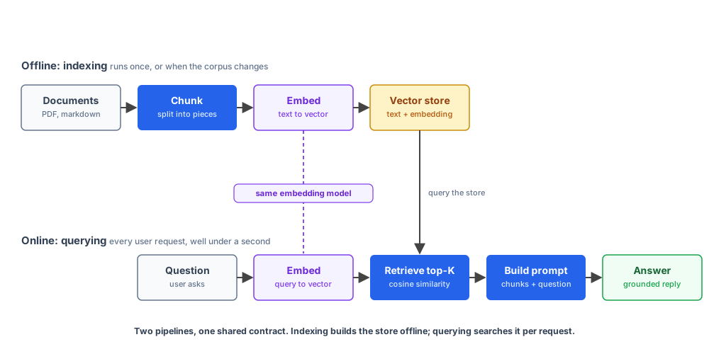
Most RAG bugs come from one confusion: which steps run when. Indexing is offline; querying is online. Mix them up and you pay in both performance and correctness. Internalise the split now and you won’t waste a week debugging why your index keeps falling out of sync with your queries.

Indexing is a batch job that runs once, or whenever your corpus changes; it can take minutes and spend tokens freely. Querying happens on every user request; it must return well under a second and pays a token cost on every call.

The two pipelines share exactly one contract: the same embedding model. If they drift apart on that one detail, the whole system silently breaks. Chapter 9 made the same point for memory recall: different embedding models on the query and the stored vectors, and the cosine scores collapse into noise.

---

Concept 5: Chunking is retrieval design

It’s tempting to treat chunking as a preprocessing detail you’ll figure out later. Don’t. How you split your documents determines what your retrieval step can discover. No reranker or prompt tweak downstream can recover information a bad chunk boundary destroyed.

Chunking is where you decide which pieces the retriever can return. Get it wrong and the rest of the system can’t help you. The two failure modes shown below are the ones you’ll actually hit in production.

The simplest chunker splits on paragraph breaks (\n\n):

function chunkByParagraph(text: string): string[] {
  return text
    .split(/\n\n+/)
    .map((p) => p.trim())
    .filter((p) => p.length > 0);
}

Three lines, and we’ll use this for the foundations build.

Two failure modes are worth seeing now.

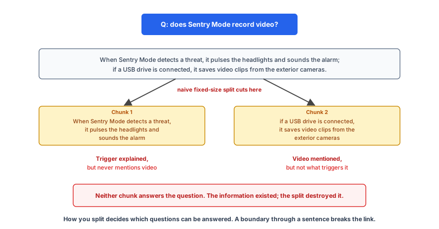
Fragmentation across boundaries. A Tesla manual section says “When Sentry Mode detects a threat, it pulses the headlights and sounds the security alarm; if a USB drive is connected, it also saves video clips from the exterior cameras.” A naive 250-character chunker splits that sentence, putting “When Sentry Mode detects a threat, it pulses the headlights and sounds the security alarm” in one chunk and “if a USB drive is connected, it also saves video clips from the exterior cameras” in the next.

The user asks “does Sentry Mode record video?” Retrieval surfaces either a chunk that explains the alarm-and-headlights response but never mentions video, or a chunk about USB-stored clips that doesn’t mention what triggers them. Neither chunk answers the question. The information existed; the chunking destroyed it.

Structure-blind splitting. Naive chunkers treat the document as a flat string. They don’t see headers, tables, list items, or code blocks as semantically meaningful boundaries. The result: a section title like ## Sentry Mode gets separated from its body, a table header gets separated from its rows, the first list item ends up in a different chunk from the rest of the list. Each fragment is grammatically valid English; none of them is useful on its own.

This is why the chapter calls chunking retrieval design: each split point decides which queries can find which answers.

Paragraph splitting (what we use in this chapter) is a reasonable default for prose-heavy corpora because paragraph boundaries usually correspond to semantic boundaries. It still breaks for long technical documents with subsections, anything with tables, code-heavy content, transcripts, and structured data exported to text.

The advanced RAG bonus chapter introduces the strategies that hold up: recursive splitting, semantic splitting, sentence-window with parent-document expansion, and layout-aware chunking. For now, run with paragraph splitting on your example corpus and notice where it works (clean prose) and where it doesn’t (anything structured).

---

Concept 6: The index pipeline in code

You’ve met embeddings, chunks, and the Two Pipelines. Time to wire them together. The index pipeline is three steps: split the document, embed each chunk, store the result. We’ll build all three in about 15 lines.

Step 1, chunk, is the function above.

Step 2 is one call to the Gemini embeddings API per chunk, with a small wrinkle:

async function embed(text: string): Promise<number[]> {
  const response = await ai.models.embedContent({
    model: "gemini-embedding-2",
    contents: `title: chunk | text: ${text}`,
    config: { outputDimensionality: 768 },
  });
  return response.embeddings![0].values!;
}

Line 1. Async helper that takes a string and returns a Promise<number[]>. The shape every chunk in your corpus will go through.

Lines 2-6. The embedContent call. model and outputDimensionality are the same as before. The new piece is the contents string: it includes a task hint (title: chunk | text:) that tells gemini-embedding-2 this text is a document chunk being indexed, not a search query.

Line 7. Pull the actual vector out of the batched response shape (embeddings![0].values!).

Unlike older Gemini embedding models, gemini-embedding-2 doesn’t have a taskType parameter; you instruct it via the content prefix. For document chunks during indexing, use the title: ... | text: ... form. For query embeddings: task: search result | query: .... Using the right prefix in each pipeline measurably improves retrieval quality.

The outputDimensionality is 768. Default is 3,072, which is more accurate but stores 4x the data; for a small corpus, 768 is enough. For production at scale, the trade-off is recall versus storage cost; the advanced RAG bonus chapter covers it.

Step 3 is store. The simplest possible “vector store” is a TypeScript array:

type Indexed = { text: string; embedding: number[]; source: string };

const index: Indexed[] = [];

for (const chunk of chunks) {
  index.push({
    text: chunk,
    embedding: await embed(chunk),
    source: filename,
  });
}

That’s it: an array of { text, embedding, source } records. For a corpus of a few hundred chunks on a developer’s laptop, this is genuinely all you need.

Any RAG running for real users needs a proper vector store: persistence, concurrent reads, sub-linear search at scale. The demo in this chapter doesn’t. An in-memory array supports the only operation you need (find the closest vector), it’s fast on thousands of chunks, and it costs nothing to set up while you’re learning the pattern.

Three steps up from the in-memory array, in order of how much you give up:

• In-memory array (this chapter). Zero ops cost. No persistence, single process, linear search. Fine for prototypes and small demos.
• SQLite + a vector extension (sqlite-vec by Alex Garcia, or SQLite-Vector from SQLite Cloud). Adds persistence and lets you embed retrieval into a single file alongside the rest of your app’s data. Still single-process, but no longer fragile across restarts. Solid middle ground for local dev or small production deployments.
• A real vector store: Postgres with pgvector, Pinecone, Qdrant, Weaviate, Chroma, Turbopuffer, and a dozen others. Sub-linear nearest-neighbour search via HNSW or similar, multi-process, replicated, observable. The right answer once you’re past tens of thousands of chunks or you need concurrent reads.

---

Concept 7: Cosine similarity

The query pipeline’s first move is “find the closest vectors to the query vector.” There are several ways to measure “close.” Cosine similarity is the standard for normalised embeddings, and you should know what it computes (and what it doesn’t) before you debug a retrieval that’s behaving strangely. Chapter 9’s cos() helper computed exactly this; now we unpack it.

Picture two arrows pointing out from the origin in some high-dimensional space. Cosine similarity asks: are these two arrows pointing in roughly the same direction? It ignores how long they are; two arrows pointing the same way score 1 even at wildly different lengths, opposite directions score -1, and perpendicular arrows score 0.

For text embeddings, “same direction” maps to “similar meaning.” Two embeddings that point the same way represent similar texts.

Compute it by hand:

function cosineSim(a: number[], b: number[]): number {
  let dot = 0;
  let normA = 0;
  let normB = 0;
  for (let i = 0; i < a.length; i++) {
    dot += a[i] * b[i];
    normA += a[i] * a[i];
    normB += b[i] * b[i];
  }
  return dot / (Math.sqrt(normA) * Math.sqrt(normB));
}

Three accumulators: dot for the dot product, normA for the squared length of a, normB for the squared length of b. One pass through the arrays: at each index, multiply the components into the dot product and accumulate squared values into the norms. This is the inner loop that gets called millions of times in production retrieval.

Then divide the dot product by the product of the lengths: two square roots and one division. The result is a number in [-1, 1]. For a few thousand chunks, calling this in a JavaScript loop is sub-millisecond on any laptop.

The full retrieval step is “compute cosine similarity against every indexed chunk, sort, take the top K”. Top-K is just the standard name for “give me the K highest-scoring items”. K is a small integer (4 in this chapter) that controls how many chunks the model sees as context.

function topK(queryEmbedding: number[], k: number): Indexed[] {
  return index
    .map((item) => ({ item, score: cosineSim(queryEmbedding, item.embedding) }))
    .sort((a, b) => b.score - a.score)
    .slice(0, k)
    .map((s) => s.item);
}

Remember that scores are relative. A score of 0.85 might be the best your embedding model can do on a query that’s poorly represented in its training. A score of 0.45 might be the best chunk in a corpus where everything is genuinely related to the query.

The useful signal is the gap between the top score and the next several. If your top four scores are 0.81, 0.79, 0.77, 0.74, retrieval is confident. If they’re 0.81, 0.42, 0.38, 0.35, only the first chunk is actually relevant; the rest are noise.

Here’s a worked similarity check. Save as code/chapter-bonus-rag/similarity-check.ts:

import { GoogleGenAI } from "@google/genai";

const ai = new GoogleGenAI({});

async function embedOne(text: string) {
  const r = await ai.models.embedContent({
    model: "gemini-embedding-2",
    contents: text,
    config: { outputDimensionality: 768 },
  });
  return r.embeddings![0].values!;
}

function cosineSim(a: number[], b: number[]) {
  let dot = 0;
  let na = 0;
  let nb = 0;
  for (let i = 0; i < a.length; i++) {
    dot += a[i] * b[i];
    na += a[i] * a[i];
    nb += b[i] * b[i];
  }
  return dot / (Math.sqrt(na) * Math.sqrt(nb));
}

const query = "What is Sentry Mode and how does it work?";
const candidates = [
  "Sentry Mode is a vehicle security feature that monitors the area around the Model 3 while it is parked and locked. When Sentry Mode detects a threat, it pulses the headlights, sounds the security alarm, and saves video clips to a connected USB drive.",
  "Use the touchscreen to control most of the vehicle's features. The 15-inch display shows the driving view, climate controls, audio, and navigation.",
  "What's the best risotto recipe?",
];

const qv = await embedOne(query);
for (const text of candidates) {
  const cv = await embedOne(text);
  console.log(cosineSim(qv, cv).toFixed(3), "|", text);
}

Output from a real run against gemini-embedding-2, dim 768 (scores are stable in practice across runs):

0.847 | Sentry Mode is a vehicle security feature that monitors the area around the Model 3 while it is parked and locked. When Sentry Mode detects a threat, it pulses the headlights, sounds the security alarm, and saves video clips to a connected USB drive.
0.662 | Use the touchscreen to control most of the vehicle's features. The 15-inch display shows the driving view, climate controls, audio, and navigation.
0.492 | What's the best risotto recipe?

The first candidate is on-topic and scores highest. The touchscreen paragraph is Tesla-adjacent but says nothing about Sentry Mode, so it lands in the middle, and the risotto question comes last.

Even the off-topic risotto query scores 0.492, not zero. Modern embedding models compress everything into the same high-dimensional space, and any two pieces of English text share enough geometry to produce non-trivial cosine similarity. Look at the gap instead. Here the gap from the on-topic chunk (0.847) to the unrelated chunk (0.492) is about 0.36, which is plenty to rank correctly.

---

Concept 8: The query pipeline in code

You’ve now seen every piece. Time to assemble them into the four-step query pipeline: embed the question, retrieve the top K, build a prompt that includes the retrieved chunks, generate the answer.

Step 1, embed the query, uses the same embed function shape with the query-task prefix:

async function embedQuery(question: string): Promise<number[]> {
  const response = await ai.models.embedContent({
    model: "gemini-embedding-2",
    contents: `task: search result | query: ${question}`,
    config: { outputDimensionality: 768 },
  });
  return response.embeddings![0].values!;
}

Same model, same dimensionality, different task prefix: that’s the Two Pipelines contract, the same embedding model on both sides.

Step 2, retrieve top-K, is the topK function from Concept 7.

Step 3 assembles the prompt. Stuff the retrieved chunks into the prompt as context, then ask the model to answer using only that context. The “using only that context” part matters; it’s how you reduce hallucination.

function buildPrompt(question: string, retrieved: Indexed[]): string {
  const context = retrieved
    .map((r, i) => `[Source ${i + 1}: ${r.source}]\n${r.text}`)
    .join("\n\n");

  return `Use the following sources to answer the question. If the answer isn't in the sources, say so.

Sources:
${context}

Question: ${question}

Answer:`;
}

Three things to notice.

Each source is labelled ([Source 1: filename]). This lets the model cite where it got each piece of the answer, and lets you trace claims back to the original.

The instruction “if the answer isn’t in the sources, say so” gives the model a structured exit. Without it, models often guess from training data when the retrieved sources don’t contain the answer.

The retrieved chunks come before the question, with the question at the end, per the lost-in-the-middle research from Chapter 2. The model attends most reliably to the start and end of the context. The question goes at the end so the model is reading it last.

Step 4 is generate. Plain generateContent call. The structured-output and tool-use machinery from Chapters 3 and 4 still works; for the foundations example we keep it simple.

async function answer(question: string): Promise<string> {
  const queryVec = await embedQuery(question);
  const retrieved = topK(queryVec, 4);
  const prompt = buildPrompt(question, retrieved);

  const response = await ai.models.generateContent({
    model: "gemini-3.5-flash",
    contents: prompt,
  });

  return response.text!;
}

Four chunks at a time (topK(..., 4)) is a reasonable starting point. More chunks means more context and potentially better answers, but more tokens spent and more lost-in-the-middle risk. Choosing K is an engineering decision we’ll revisit in the advanced RAG bonus chapter.

The full script below logs the top scores to stderr as a [retrieve] line, and that line is more useful than it looks. Each number is one retrieved chunk’s cosine similarity to the query, best first: four chunks, four scores. Three patterns to watch for. The example scores are real runs against the Tesla manual corpus we index below; the absolute values are specific to the embedding model. gemini-embedding-2 compresses everything into roughly 0.4–0.85, so judge each run by the gaps between the four scores rather than by a fixed threshold.

Confident retrieval: top scores are high and tightly clustered.

[retrieve] top scores: 0.827, 0.766, 0.765, 0.743

The corpus has the answer; multiple chunks are reinforcing each other. The model’s answer should be solid. This run was “how do I open the charge port?”, which the manual covers several times over.

Honest miss: the scores are flat and barely above what an average chunk would get.

[retrieve] top scores: 0.533, 0.531, 0.524, 0.522

This is “what is the best recipe for sourdough bread?” asked against a car manual. It doesn’t look dramatic, and that’s the trap: with this embedding model even a completely unrelated chunk scores around 0.45, so a genuine miss never shows a score near zero. What gives it away is the shape: all four scores sit within 0.011 of each other, with nothing standing out. Nothing in the corpus is a real match, so the model should refuse, and your prompt’s “if the answer isn’t in the sources, say so” instruction is what makes that happen.

Lone hit: one clear score, then a drop to the flat zone.

[retrieve] top scores: 0.733, 0.656, 0.649, 0.647

One chunk matched; the other three are filler. This pattern has two readings, and the scores alone can’t tell you which you’ve got. The benign one: the answer lives in exactly one paragraph. This run was “how many litres of washer fluid does the reservoir hold?”, where a single chunk holds the capacity figure (3.2 litres) and the model answered correctly from it. The dangerous one: the top chunk merely shares vocabulary with the question without containing the answer, and with nothing to contradict it the model latches on and produces a fluent wrong answer. A lone hit is the one pattern where you should check the retrieved chunk before trusting the output.

Reading these patterns spares you the “model sounds confident but is wrong” debugging sessions. Two minutes with the scores can save you an hour of staring at outputs.

---

Putting it all together

Here’s the whole minimum-viable RAG, end to end: a simplified version of code/chapter-bonus-rag/rag.ts (the repo file adds one extra, covered after the listing). The corpus is a single PDF (the Tesla Model 3 owner’s manual, dropped at corpus-pdf/model3-manual.pdf), so the index pipeline adds one extraction step compared to the simpler markdown case:

import { GoogleGenAI } from "@google/genai";
import { readFileSync, readdirSync } from "node:fs";
import { join, extname } from "node:path";
import { PDFParse } from "pdf-parse";

const ai = new GoogleGenAI({});

type Indexed = { text: string; embedding: number[]; source: string };
const index: Indexed[] = [];

function chunkByParagraph(text: string): string[] {
  return text
    .split(/\n\n+/)
    .map((p) => p.trim())
    .filter((p) => p.length > 40); // drop very short fragments (page numbers, headers)
}

async function extractText(filePath: string): Promise<string> {
  if (extname(filePath).toLowerCase() === ".pdf") {
    const data = readFileSync(filePath);
    const parser = new PDFParse({ data });
    const result = await parser.getText();
    await parser.destroy();
    return result.text;
  }
  return readFileSync(filePath, "utf-8");
}

async function embedAs(role: "doc" | "query", text: string): Promise<number[]> {
  const prefix = role === "doc"
    ? `title: chunk | text: ${text}`
    : `task: search result | query: ${text}`;
  const response = await ai.models.embedContent({
    model: "gemini-embedding-2",
    contents: prefix,
    config: { outputDimensionality: 768 },
  });
  return response.embeddings![0].values!;
}

function cosineSim(a: number[], b: number[]): number {
  let dot = 0;
  let normA = 0;
  let normB = 0;
  for (let i = 0; i < a.length; i++) {
    dot += a[i] * b[i];
    normA += a[i] * a[i];
    normB += b[i] * b[i];
  }
  return dot / (Math.sqrt(normA) * Math.sqrt(normB));
}

// --- Index pipeline ---
const corpusDir = "./corpus-pdf";
for (const file of readdirSync(corpusDir)) {
  const ext = extname(file).toLowerCase();
  if (ext !== ".pdf" && ext !== ".md") continue;
  const text = await extractText(join(corpusDir, file));
  for (const chunk of chunkByParagraph(text)) {
    index.push({
      text: chunk,
      embedding: await embedAs("doc", chunk),
      source: file,
    });
  }
  console.error(`[index] indexed ${file}`);
}
console.error(`[index] ${index.length} chunks total`);

// --- Query pipeline ---
const question = process.argv.slice(2).join(" ");
if (!question) {
  console.error('Usage: npm run rag -- "your question"');
  process.exit(1);
}

const queryVec = await embedAs("query", question);
const retrieved = index
  .map((item) => ({ item, score: cosineSim(queryVec, item.embedding) }))
  .sort((a, b) => b.score - a.score)
  .slice(0, 4);

console.error(
  `[retrieve] top scores: ${retrieved.map((r) => r.score.toFixed(3)).join(", ")}`
);

const context = retrieved
  .map((r, i) => `[Source ${i + 1}: ${r.item.source}]\n${r.item.text}`)
  .join("\n\n");

const response = await ai.models.generateContent({
  model: "gemini-3.5-flash",
  contents: `Use the following sources to answer the question. If the answer isn't in the sources, say so.

Sources:
${context}

Question: ${question}

Answer:`,
});

console.log(response.text);

Lines 1-4. Imports. SDK plus Node’s file-system helpers and the pdf-parse library for extracting text from PDFs. pdf-parse is a small dependency that wraps Mozilla’s PDF.js under the hood; install it with npm install pdf-parse.

Line 6. Standard client construction.

Lines 8-9. The in-memory vector store: a type Indexed = { text, embedding, source } and an empty array. This is the chapter’s “vector store.” Production swaps this out for pgvector or similar; for the demo, the array is the index.

Lines 11-16. chunkByParagraph from Concept 5. Splits on \n\n+, trims, drops fragments under 40 characters. The length filter matters more here than in the markdown case: PDF text extraction produces stray page numbers, section headers, and orphaned punctuation as “paragraphs,” and you don’t want those polluting the index.

Lines 18-27. extractText is the PDF-specific addition. If the file is a PDF, instantiate PDFParse, call getText(), return the extracted plain text. Otherwise read the file as UTF-8 text. The rest of the pipeline doesn’t care what format the source was; once you have a string, everything from chunking down is the same.

Lines 29-39. embedAs is the chapter’s only meaningful indirection: embed with the right task prefix depending on whether you’re indexing a document chunk ("doc") or embedding a query ("query"). Same embedContent call shape, different prefix.

Lines 41-51. cosineSim from Concept 7.

Lines 53-68. The index pipeline. Walk ./corpus-pdf/, extract text from every PDF (or markdown file) you find, chunk each by paragraph, embed each chunk with the doc prefix, push { text, embedding, source } into the index. The PDF extraction step adds a few seconds on first run for a 300-page manual; the embedding calls are what dominate after that.

Lines 71-75. CLI argument handling. process.argv.slice(2).join(" ") joins everything after the script name into one question string.

Line 77. Embed the question with the query prefix. Different prefix from the docs, same model and dimensionality.

Lines 78-81. Retrieval. Map every indexed chunk to { item, score } where score is cosine similarity against the query vector, sort by score descending, take the top 4.

Lines 83-85. Log the top scores to stderr so you can see whether retrieval was confident (close scores at the top) or shaky (big gaps).

Lines 87-89. Format the retrieved chunks into a Sources: block tagged with [Source N] markers.

Lines 91-101. The generation call. The prompt embeds the sources block and the user question into a single user message. The “If the answer isn’t in the sources, say so” instruction is the chapter’s grounding guard: it tells the model to refuse rather than fabricate when the sources don’t cover the question.

Drop the Tesla Model 3 owner’s manual PDF at code/chapter-bonus-rag/corpus-pdf/model3-manual.pdf and run it:

$ npm run rag -- "What is Sentry Mode?"

[index] indexed model3-manual.pdf
[index] 321 chunks total
[retrieve] top scores: 0.788, 0.754, 0.695, 0.688
Sentry Mode is an intelligent vehicle security system for the Tesla
Model 3 that monitors the area around the vehicle for suspicious
activity or possible threats when the car is locked and in Park.
When enabled, the vehicle's cameras and sensors remain powered on.
If a threat or "jerky movement" (such as towing or shaking) is
detected, the system pulses the headlights, sounds the alarm,
displays a message on the touchscreen informing those outside that
cameras may be recording, sends an alert to the owner's mobile app,
and saves footage of the event to a USB drive (if one is installed).

For Sentry Mode to save video footage, a properly formatted USB drive
must be inserted into a USB port (preferably the one in the glove box)
and the Dashcam feature must be enabled. If no USB drive is present,
the vehicle still sends alerts to the mobile app but does not record
video. Sentry Mode is disabled by default; it can be enabled via voice
commands ("Sentry on", "Keep Tesla safe"), the mobile app, or the
vehicle's touchscreen.

Sentry Mode is not available when the vehicle is in Low Power Mode,
and power consumption may increase when the mode is active. It does
not capture audio.

That’s working RAG in about 90 lines including the PDF extraction step: no vector database, no framework, no cloud service beyond Gemini itself.

One practical thing the version in the repo carries that the listing above doesn’t: an on-disk embedding cache. The chapter’s snippet rebuilds the index on every run, which re-embeds all 321 chunks against gemini-embedding-2 every time you re-run the script. That’s fine the first time and wasteful every time after, both in seconds and in embedding tokens.

The full rag.ts in the repo writes the indexed { text, embedding, source } array to cache/embeddings.json once (its first-run index line reads [index] 321 chunks total; wrote cache to ./cache/embeddings.json), then on subsequent runs checks whether the cache is newer than the source PDF and, if so, loads from cache instead of re-embedding. Invalidation is mtime-based: edit or replace a PDF in corpus-pdf/ and the next run notices the source is newer than the cache and rebuilds.

The rest of the pipeline is unchanged, but the per-run cost of indexing drops from “embed 321 chunks” to “read one JSON file.” You end up with the same in-memory index after either path; it’s just cheaper to develop against.

Action

1. Set up code/chapter-bonus-rag/, install @google/genai and pdf-parse, add .env. Download the Tesla Model 3 owner’s manual PDF and drop it at corpus-pdf/model3-manual.pdf. Run rag.ts with three questions: one whose answer is there (e.g. “What is Sentry Mode?”), one partially there, one missing entirely (e.g. “How do I deploy a Hono server?”).
2. Drop your own PDF or markdown into corpus-pdf/, re-run, and watch the [retrieve] top scores line. The gap between the top score and the rest is your honesty signal.
3. Compare the repo’s assistant.ts to the Chapter 5 (AGENTS.md-only) version. It keeps the developer persona in systemInstruction but swaps skills-in-the-system-prompt for retrieved sources in the user message, with [Source N] citation rules. Ask both the same question and compare the answers.

---

Next up, the advanced RAG bonus chapter: RAG that actually works. The chunking strategies that beat paragraph-splitting, why you need a reranker, when hybrid search wins, which vector stores are worth their complexity, and how to evaluate RAG quality without staring at outputs all day.