RAG that actually works

What you’ll build

The pipeline from the RAG bonus chapter works on the example corpus. Try it on a real one and you’ll hit at least three problems within an hour.

Retrieval misses obvious answers. The user asks “how do I stop the cabin from frying in the summer?” The Tesla manual says “Cabin Overheat Protection prevents the cabin from getting too hot in scorching ambient conditions.” Dense embeddings get this one. You also discover three queries where dense doesn’t, and they all involve specific named features like Sentry Mode, Camp Mode, or Pet Mode that BM25 would have nailed.

Top-K is wrong. The retriever surfaces four chunks: two are great, two are tangentially related and dilute the model’s attention, and answer quality drops.

And you don’t know if your changes are helping. You tweak chunk size, rerun a few queries, the answers seem better, but you’re not sure. Two weeks later you’ve made twelve changes and have no idea which ones moved the needle.

Each of these has a known fix. Five upgrades over the RAG bonus chapter, in the order they pay off:

1. Better chunking. Recursive splitting, sentence-window with parent-doc, semantic chunking, layout-aware. Paragraph splitting is the cheapest correct option; these do better.
2. Hybrid search. Sparse (BM25) plus dense (embeddings), combined with Reciprocal Rank Fusion. A measurable, corpus-dependent recall lift over dense alone, biggest when queries name specific features.
3. Reranking. A second-pass cross-encoder reorders the top candidates. The biggest single quality lift in the chapter; the size varies by corpus and metric, so measure it (Concept 7 has the honest numbers).
4. Real vector store. When the in-memory array stops being enough.
5. Evaluation. RAGAS-style metrics (faithfulness, answer relevance, context precision, context recall) so you measure quality changes instead of guessing.

I’ll thread these through one shape: the Retrieval Funnel. Retrieve broadly, narrow with reranking, ground generation in the survivors. The underlying pattern is the established two-stage retrieve-and-rerank flow (Pinecone’s “Rerankers and Two-Stage Retrieval”, the Re2G paper, every major vector store’s docs); the funnel name is the chapter’s working label.

RAG design decisions are mostly about how wide the funnel opens, where it narrows, and how aggressively.

If you skipped the RAG bonus chapter, go back. The code in this chapter assumes you understand embeddings, the Two Pipelines, cosine similarity, and the basic chunk-embed-store-retrieve-augment-generate flow.

One note on reading order: Concepts 1 to 7 build the production-shape RAG you’ll deploy, and the second half of Concept 8 defines the store that pipeline runs on (SQLite + sqlite-vec + FTS5), so read that part too. Concept 8’s store survey and Concept 9 are operations material, worth skimming on a first read and returning to when something specific breaks. Concept 10 points back to Chapter 10 for evaluation.

---

Concept 1: The Retrieval Funnel

The RAG bonus chapter’s pipeline collapsed retrieval into one step: top-K by cosine similarity. That’s fine for foundations and inadequate for anything you’d ship. Production retrieval has stages with different optimisation targets. If you don’t know what each stage is for, you can’t tell which one is failing when the answer is wrong.

The funnel shape is literal. Anything that might be relevant pours in at the wide top, a sieve in the middle catches the good candidates and lets the noise drain through, and only the best survivors reach the model at the narrow bottom. A wide top means high recall (don’t miss the answer); a narrow bottom means high precision (don’t hand the model junk). The sieve is reranking, and you have to opt in.

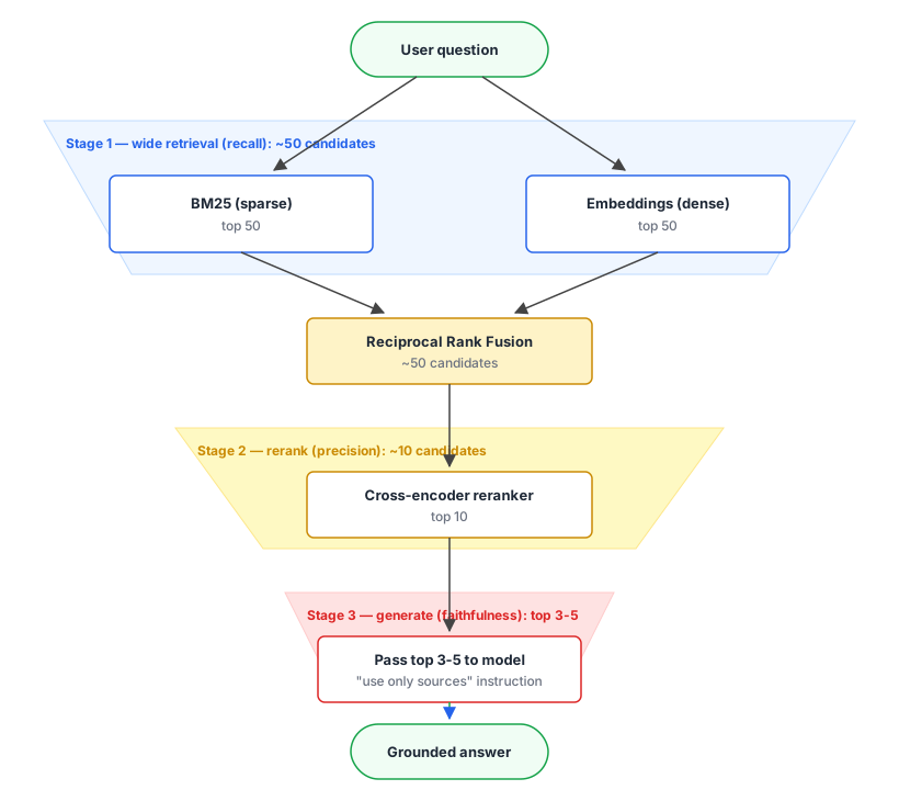
Three numbers worth memorising as a starting point:

• Retrieve about 50 candidates with hybrid search (cast a wide net for recall).
• Rerank to the top 5 to 10 with a cross-encoder (narrow for precision).
• Pass 3 to 5 to the generation prompt (constrain context for faithfulness).

Treat them as reasonable defaults to tune per corpus; the shape matters more than the exact numbers.

Common confusion: “more retrieval = better answer.” Past a certain point each extra chunk dilutes the model’s attention without adding signal. The funnel exists because precision and recall pull in different directions; you need a wide net for recall and a narrow handoff for precision.

---

Concept 2: Recursive chunking

Paragraph splitting from the RAG bonus chapter is the cheapest correct option. It breaks on long technical documents (huge chunks if a section has no paragraph breaks), tables (split mid-row), and structured content (heading separated from body). Recursive chunking is the production default that handles all three by trying boundaries from largest to smallest.

The shape: try the big boundaries first (sections, then paragraphs). Fall back to smaller ones (sentences, words). Each fallback is coarser than the last, but the result always lands in your target size range and respects document structure where possible.

function recursiveSplit(
  text: string,
  maxChars = 1000,
  separators = ["\n## ", "\n### ", "\n\n", ". ", " "]
): string[] {
  if (text.length <= maxChars) return [text];

  for (const sep of separators) {
    if (text.includes(sep)) {
      const parts = text.split(sep);
      const out: string[] = [];
      let current = "";
      for (const part of parts) {
        const candidate = current ? `${current}${sep}${part}` : part;
        if (candidate.length <= maxChars) {
          current = candidate;
        } else {
          if (current) out.push(current);
          current = part.length > maxChars
            ? recursiveSplit(part, maxChars, separators).join("\n")
            : part;
        }
      }
      if (current) out.push(current);
      return out;
    }
  }
  return [text];
}

Three parameters: the text, the target max size in characters, and the priority-ordered separators. The defaults are tuned for Markdown. The base case returns the text untouched if it already fits.

Otherwise the function tries each separator in order. For the first one present in the text, split there, then re-pack the parts: greedily combine consecutive parts until adding the next one would overflow maxChars. Push the current pack and start a new one.

The recursive case kicks in when a single part is itself bigger than maxChars. Recurse on that part with the remaining separators. This is what guarantees no chunk ever exceeds the limit.

The trick is in the trial order. A long Markdown section gets split at ## first. If a single section is still too big, split at \n\n. If a paragraph is somehow too big, split at . . Words last. The result respects the document’s structure where possible.

Even with good boundaries, a fact that sits on a chunk boundary can get split in half. The fix is overlap: include the last N characters of the previous chunk at the start of the next.

function withOverlap(chunks: string[], overlapChars = 150): string[] {
  return chunks.map((chunk, i) => {
    if (i === 0) return chunk;
    const tail = chunks[i - 1].slice(-overlapChars);
    return `${tail} ${chunk}`;
  });
}

Typical overlap is 10 to 20% of chunk size. Bigger overlap means duplicate content (more tokens to embed and retrieve). Smaller overlap means context loss at boundaries.

Common confusion: “tokens, not characters.” You might wonder why the size cap is in characters instead of tokens. Tokens are what the model and embedding API actually count. Two reasons to cap by character anyway: tokenising every candidate chunk during recursion is expensive, and characters are a tight enough proxy (English averages about four characters per token, so 1,000 chars is roughly 250 tokens). For specialist corpora (code, non-English) you’d switch to a token-based cap.

Recursive plus overlap is the production default for prose; it serves about 80% of corpora well.

Common confusion: “the defaults are good defaults.” On real corpora, “1,000 characters with 150 character overlap” is a starting point, not a recipe. The right maxChars depends on how dense your information is per character (a recipe blog has different signal density than a legal contract); the right overlapChars depends on how often facts span chunk boundaries on your specific corpus.

Expect to run an eval suite on three or four (chunk size, overlap) combinations before you settle. The improvement from “default 1,000/150” to “tuned for your corpus” is often 5-10 points on context recall. Don’t ship the defaults blind. (Chapter 10 builds the suite.)

---

Concept 3: Sentence-window with parent-document retrieval

There’s a tension in chunk size. Small chunks embed sharply (the embedding signal is concentrated). Large chunks give the model more context to reason from. Recursive chunking with overlap hits a compromise. Sentence-window with parent-doc retrieval picks both: index small, return large.

You search by sentence and return the paragraph: the sentence’s embedding is the sharper match signal, and the paragraph carries the context the model actually answers from.

To make that concrete, take a paragraph from the Model 3 manual that mixes five facts about Sentry Mode:

[paragraph P1]
S1: Sentry Mode monitors the area around the Model 3 when the vehicle is
    locked and in Park.
S2: When a threat is detected, the system pulses the headlights, sounds
    the alarm, and displays a warning on the touchscreen.
S3: Sentry Mode saves video clips to a properly formatted USB drive
    inserted in the glove-box USB port; if no drive is present, no video
    is recorded.
S4: Camera-Based Detection uses the exterior cameras in addition to the
    physical sensors to spot security events.
S5: Sentry Mode automatically disables in Low Power Mode and at any
    Excluded Location (Home, Work, or saved Favorites).

A user asks: “Does Sentry Mode work if I haven’t put a USB drive in the car?”

Embed the whole paragraph as one vector. That vector represents an averaged direction across “monitoring / threat response / USB recording / camera detection / disable conditions.” The query matches it at, say, cosine 0.62. A separate paragraph on Dashcam (which also writes video to USB) might score 0.58. The two are close enough to be ambiguous.

Embed each sentence separately and S3 (“Sentry Mode saves video clips to a properly formatted USB drive… if no drive is present, no video is recorded”) becomes a vector pointing sharply at USB and recording. The query sits next to it. Cosine similarity climbs to roughly 0.81 on S3; S1 is ~0.40, S2 ~0.35, the Dashcam sentences lower still. The match has gone from ambiguous to obvious.

But you don’t want the writer to receive only S3. The sentence in isolation (“Sentry Mode saves video clips to a properly formatted USB drive…”) doesn’t tell the user what does still happen without the drive. Hand the writer the parent paragraph P1 and the answer composes itself: “Without a USB drive, Sentry Mode still monitors and still triggers the alarm response on a threat, but it won’t record any video [c25-S3]. Insert a drive and clips save automatically.”

The trick that closes the loop: index S1-S5 separately, but tag each with parentId: P1. At query time the top match is S3 (sharp); look up its parent and return P1 to the writer. The sentence is good at being found; the paragraph is good at being read.

The umbrella name for the pattern is small-to-big retrieval, popularised by Sophia Yang’s 2023 write-up of LlamaIndex’s small-to-big retrievers. LangChain ships it as ParentDocumentRetriever, and LlamaIndex ships SentenceWindowNodeParser for the sentence-window variant.

type ChunkWithParent = {
  text: string;             // small sentence-level chunk for embedding
  parent: string;           // larger paragraph or section returned to the model
  parentId: string;         // dedupe if multiple sentences have the same parent
};

At index time, split the document into paragraphs (the parents). Within each paragraph, split into sentences (the searchable units). Embed the sentences. Store both. At query time, embed the query, find the top-K matching sentences, then dedupe by parentId and return the parents to the model.

Common confusion: “why not embed paragraphs?” You might think embedding the parent directly would skip the indirection. It would also blunt the embedding, exactly as the Sentry Mode example showed: a paragraph that mentions five things produces a vector that’s a weighted average of all five, harder to discriminate against, while a sentence that mentions one thing points sharply at it.

Use sentence-window when answers are scattered across long documents and embedding-on-paragraphs is too coarse to discriminate. Skip it for short documents where paragraph-level chunking already retrieves cleanly.

---

Concept 4: Semantic chunking

Recursive chunking respects structural boundaries (headings, paragraphs). Semantic chunking respects meaning boundaries: split where the topic shifts, not where the formatting suggests it. Useful for transcripts, support-chat logs, anything not authored as prose with reliable structural cues.

The mechanism: embed each sentence, compute cosine distance between adjacent sentence embeddings, insert a chunk boundary wherever the distance exceeds a threshold. The threshold is what you tune per corpus. Popularised by Greg Kamradt in late 2023 and early 2024, the technique now ships as LangChain’s SemanticChunker (which exposes four threshold strategies: percentile, standard deviation, interquartile, gradient) and LlamaIndex’s semantic chunking pack.

Semantic chunking is more expensive than recursive (you embed every sentence, then compute pairwise distances) and the boundary detection is fiddly to tune. It pays off on documents where structural cues are unreliable. For typical Markdown or HTML docs, recursive splitting is cheaper and as good.

Common confusion: “more sophisticated must be better.” On well-structured corpora, recursive chunking matches semantic chunking on retrieval quality at a fraction of the indexing cost. The 2024 arXiv paper Is Semantic Chunking Worth the Computational Cost? tested it across benchmarks and found the lift is small to absent on most corpora. Save semantic chunking for corpora where structural splits demonstrably break the retrieval.

---

Concept 5: Layout-aware chunking

When your source has structure that carries meaning (Markdown headings, HTML sections, tables, code blocks), naive character splitting destroys it. Two failure modes you’ll see immediately if you don’t respect layout.

Tables get split mid-row. A pricing table with five tiers becomes three half-tables across three chunks, none of which retrieves cleanly when the user asks “what’s the price for the Pro tier?”

Section titles get separated from their bodies. A heading like ## Bank trading ends up in chunk N, the actual rules live in chunk N+1. Retrieval pulls the body, the model sees the rules with no context about what topic they belong to.

The fix is to parse the source format before chunking and treat structural elements (headings, tables, code blocks, list items) as atomic where possible. For Markdown specifically, the cheap win is using \n## and \n### as primary separators in recursive splitting (which the recursive code above already does). For HTML, parse with a real HTML parser and chunk per <section> or <article>. For PDFs with tables and figures, you’ll want a layout-aware document parser (Unstructured.io, LlamaParse, Reducto, or IBM’s open-source Docling) before chunking.

Common confusion: “the embedding model handles structure.” Embedding a half-table produces an embedding for half a table. You’re better off keeping the table whole as one chunk (even if it overflows your usual size cap) than splitting it.

Structure carries meaning, so parsing the source is part of chunking.

---

Pick chunking by corpus shape

A quick rule of thumb you can apply tomorrow:

• Plain prose (blogs, articles, transcripts): recursive with paragraph-first splits, 800 to 1,200 char chunks, 10 to 15% overlap.
• Structured docs (Markdown wikis, API docs): recursive with heading-first splits.
• Highly heterogeneous mixed content (PDFs with tables, images, code): layout-aware parser first, then recursive within each parsed block.
• Short, fragmented sources (FAQs, support tickets): treat each Q-A pair or ticket as one chunk. Don’t split.
• Long answers scattered across long documents: sentence-window with parent-doc retrieval.

Framework defaults run large. LangChain’s TextSplitter ships at 4,000 characters with a 200-char (5%) overlap. LlamaIndex’s SentenceSplitter at 1,024 tokens (~4,000 chars) with a 200-token (~20%) overlap. Most practitioners tune down. A common landing zone for embedding-based retrieval is 500 to 1,500 characters with 10-20% overlap, because smaller chunks embed more sharply (the same point Concept 3 made about sentences). An eval suite (Chapter 10) tells you which way to err on your corpus.

---

Concept 6: Hybrid search with RRF

The RAG bonus chapter introduced sparse and dense retrieval as a trade-off. The practical answer is to run both and combine the rankings rather than pick one. The lift is real and the implementation is simple, which is why this is the second-cheapest big quality win after better chunking.

Hybrid search runs sparse and dense retrieval in parallel and fuses the rankings. A document that scores high on both lists is one that mentions the user’s specific tokens and is about the topic. Either method alone misses one half of that signal.

A user asking your Tesla manual corpus: “What does Pet Mode do?”

Dense retrieval looks at the meaning. It finds sections about cabin climate control in general. It might miss that the specific phrase “Pet Mode” is exactly what the user named, because the embedding flattens the literal phrase into a generic “cabin climate / comfort” signal. Sparse retrieval (BM25) sees “Pet Mode” as a literal token sequence and ranks any document that contains it at the top, regardless of whether the surrounding text actually explains the feature.

Run both, combine the rankings, and you get the chunk that’s both about the climate system and mentions the exact feature name.

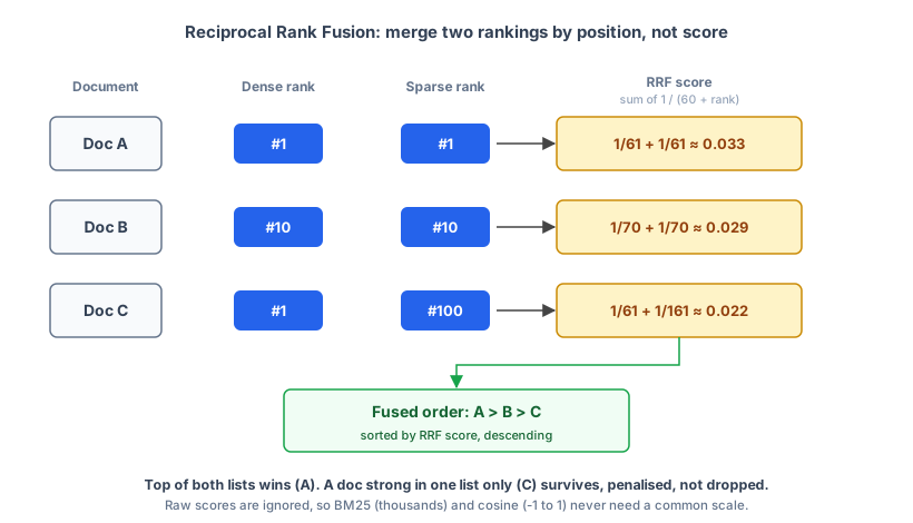
Reciprocal Rank Fusion (RRF) is the standard way to combine the two rankings. Why not just add the scores? Because BM25 scores are unbounded and corpus-dependent (magnitudes around 9 to 10 on this corpus) while cosine scores live between -1 and 1. Summing them just lets the bigger number dominate. RRF sidesteps that by ignoring scores entirely and only looking at position in each ranking.

The formula is one line: for every document, add up 1 / (k + rank) for each list it shows up in. k is a constant that softens the curve so a document at rank 1 doesn’t completely drown out a document at rank 5. The convention is k = 60, which is what the original RRF paper used (Cormack, Clarke & Buettcher (2009 SIGIR)).

Three documents, walked through:

Document	Rank in dense	Rank in sparse	RRF score
A	1	1	1/61 + 1/61 ≈ 0.033
B	10	10	1/70 + 1/70 ≈ 0.029
C	1	100	1/61 + 1/161 ≈ 0.022

Document A wins because it’s near the top of both lists. Document C is strong in dense but weak in sparse, and it scores noticeably lower than A even though they share rank 1 in dense. The doc that’s strong in only one list still ranks; it’s penalised, not eliminated.

function rrf<T>(
  rankings: T[][],
  keyFn: (item: T) => string,
  k = 60
): { item: T; score: number }[] {
  const scores = new Map<string, { item: T; score: number }>();
  for (const ranking of rankings) {
    ranking.forEach((item, rank) => {
      const key = keyFn(item);
      const existing = scores.get(key);
      const contribution = 1 / (k + rank + 1);
      if (existing) {
        existing.score += contribution;
      } else {
        scores.set(key, { item, score: contribution });
      }
    });
  }
  return [...scores.values()].sort((a, b) => b.score - a.score);
}

Lines 1-5. The function signature. Generic over the item type T so it works with any kind of ranked entry. Takes a list of rankings (each itself a list), a keyFn that extracts a stable key from an item (used to merge duplicates across rankings), and the k constant.

Line 6. const scores = new Map<...> keeps a running total per key. Map (not plain object) so we get insertion-order iteration and don’t trip on prototype keys.

Lines 7-15. Iterate every ranking. For each item at position rank (0-indexed), compute its contribution as 1 / (k + rank + 1): position 0 contributes 1/61 with k=60, position 1 contributes 1/62, and so on. Add the contribution to the existing entry for that key, or create a new one.

Line 19. Sort by total score, descending. That’s the whole algorithm.

Using wink-bm25-text-search for sparse and the dense pipeline from the RAG bonus chapter:

import bm25 from "wink-bm25-text-search";

const sparse = bm25();
sparse.defineConfig({ fldWeights: { text: 1 }, bm25Params: { k1: 1.2, b: 0.75 } });
sparse.definePrepTasks([
  // tokenizer pipeline: lowercase, split on whitespace, remove punctuation
]);

// Index
for (const chunk of chunks) {
  sparse.addDoc({ text: chunk.text }, chunk.id);
}
sparse.consolidate();

// Query
const sparseResults = sparse
  .search(question)
  .map(([id, score]) => ({ id, score }));

const queryVec = await embedAs("query", question);
const denseResults = chunks
  .map((chunk) => ({ id: chunk.id, score: cosineSim(queryVec, chunk.embedding) }))
  .sort((a, b) => b.score - a.score)
  .slice(0, 50);

const hybrid = rrf(
  [sparseResults, denseResults],
  (item) => String(item.id)
);

Line 1. Import the Node-friendly BM25 implementation. wink-bm25-text-search ships an in-memory index, no native dependencies.

Lines 3-7. bm25() constructs an index. defineConfig sets BM25’s two tunable parameters (k1, b) and the per-field weight. definePrepTasks is the tokenizer pipeline: lowercase, split on whitespace, strip punctuation. The pipeline runs on every doc you add and every query you search.

Lines 10-13. Index every chunk by id. consolidate() finalises the index after adds; you can’t search until you’ve called it.

Lines 16-18. The sparse pass. sparse.search(question) returns [id, score] tuples, not objects, so map each tuple into an object carrying the id the fusion step keys on.

Lines 20-24. The dense pass, built from the RAG bonus chapter’s pieces: embedAs embeds the query, cosineSim scores every chunk against it, sort descending, keep the top 50.

Lines 26-29. Fuse the two ranked lists with rrf. The keyFn returns each item’s id as a string so the same chunk found by both methods gets one merged score.

sparseResults and denseResults use entirely different scoring scales. RRF only looks at rank position, so the scale mismatch doesn’t matter.

One honest note: the snippet above is the concept in isolation. The chapter’s running build (Concept 8) gets BM25 from SQLite’s FTS5 instead of wink, so the companion repo has no wink dependency; hybrid-search.ts is the runnable equivalent of this wiring.

In practice you’ll retrieve maybe 50 candidates from each method, fuse with RRF, and pass the top of the fused list to reranking. Concept 1’s default handoff is about 50; the chapter’s build trims it to 10 to keep the local cross-encoder fast. The two retrieval methods catch different misses, so the fused ranking holds up better than either alone.

Common confusion: “I’ll just average the scores.” A weighted average of BM25 and cosine scores fails for the scale reason above: naive averaging lets BM25 dominate every result.

Even after normalisation, the distribution shapes are different enough that one method’s high-confidence band overlaps the other’s noise band. RRF avoids the whole problem by working on ranks. Use it.

For corpora that are small (a few hundred chunks), well-structured, and use consistent terminology, dense alone is often within 5% of hybrid quality. The added complexity isn’t worth it. For corpora with named entities (named cards, characters, expansions), specific rule terms, or version-specific identifiers, hybrid is a step change. Don’t ship without it.

---

Concept 7: Reranking

Hybrid search casts a wide net. A wide net catches a lot of weakly-relevant junk along with the gold. Reranking is the second pass that promotes the truly relevant items. It’s the biggest single quality lift in this chapter and the most commonly skipped step.

Before going deeper, pin down how this differs from Concept 6. Hybrid + RRF and reranking sit at different stages of the funnel and do different work:

	Hybrid + RRF (Concept 6)	Reranking (this concept)
Pipeline stage	Wide retrieval	Narrowing filter
Input	Query	Query + ~50 candidates from retrieval
Looks at	Rank positions only	Full content of each (query, candidate) pair
Cost	Cheap (embedding + BM25 lookups, then merge ranks)	Expensive (one model call per pair)
Output	~50 candidates	Top ~5-10
What it catches	Token matches the dense embedding flattened away	Candidates that look relevant but aren’t

The two are complementary. Hybrid casts the wide net so the right answer ends up somewhere in the top 50. Reranking is what pulls it to position 1. Skip hybrid and recall drops (the embedding misses literal token matches); skip reranking and precision drops (the model gets 50 candidates that all look relevant, including 40 that aren’t).

The retriever in the funnel so far is a bi-encoder: query and documents got embedded separately, then compared by vector similarity: fast, but coarse. A reranker is a different shape of model called a cross-encoder. It processes the query and each candidate together and scores them jointly. Slower per item, much more accurate per item, because the model sees both inputs at once. The funnel pays this cost only on the top 50 candidates from retrieval, not the whole corpus.

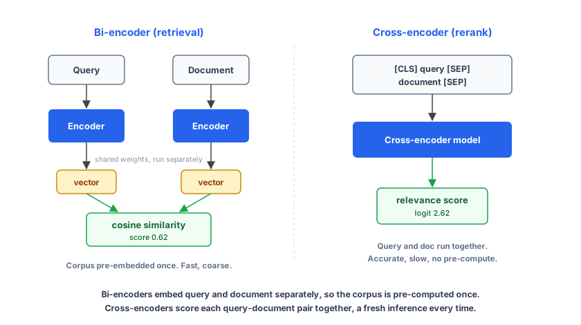
The trade-off is exactly why the funnel exists. Cross-encoding a million documents per query is too slow; cross-encoding the top 50 candidates from your retriever is fast enough. That’s reranking.

The lowest-friction way to wire a reranker is to run it locally. Transformers.js has cross-encoder weights in ONNX format that load straight into Node, no vendor signup, no API key. The first run downloads the model (around 280 MB for Xenova/bge-reranker-base) and caches it; later runs load from disk.

import { AutoTokenizer, AutoModelForSequenceClassification } from "@huggingface/transformers";

const tokenizer = await AutoTokenizer.from_pretrained("Xenova/bge-reranker-base");
const model = await AutoModelForSequenceClassification.from_pretrained("Xenova/bge-reranker-base");

async function rerank(
  query: string,
  documents: { id: string; text: string }[],
  topN = 10
): Promise<{ id: string; score: number }[]> {
  const inputs = tokenizer(
    documents.map(() => query),
    { text_pair: documents.map((d) => d.text), padding: true, truncation: true }
  );
  const { logits } = await model(inputs);
  const scores: number[] = Array.from(logits.data as Float32Array);
  return documents
    .map((d, i) => ({ id: d.id, score: scores[i] }))
    .sort((a, b) => b.score - a.score)
    .slice(0, topN);
}

Line 1. Two imports from @huggingface/transformers: AutoTokenizer for tokenising query/doc pairs, AutoModelForSequenceClassification for the cross-encoder model itself.

Lines 3-4. Load both off Hugging Face. Xenova/bge-reranker-base is the ONNX-converted variant of the canonical BAAI/bge-reranker-base model, downloaded and cached on first run.

Lines 6-10. Function signature. Takes a query string, an array of { id, text } documents, and a topN cap.

Lines 11-14. Tokenise. documents.map(() => query) repeats the query string once per document; text_pair carries the corresponding doc. The tokenizer pairs them into the [CLS] query [SEP] doc [SEP] shape the cross-encoder expects, with padding and truncation.

Line 15. Run the model. logits is a tensor with one logit per (query, doc) pair.

Line 16. Pull the logits out as a JS number array.

Lines 17-20. Pair each document with its score, sort descending, return the top topN. Higher logit = more relevant; the values are unbounded (negative is normal for irrelevant pairs).

The full pattern: tokenise each (query, doc) pair as a sequence pair (the text_pair arg), run the model, read one logit per pair from logits.data, and sort. The logits aren’t probabilities, so sorting is the only thing you do with them.

Alternatives worth knowing:

• Hosted APIs: Cohere Rerank, Jina Reranker, Voyage Rerank. One HTTP call each, no model to host, vendor relationship and per-query cost.
• Open-weight, self-hosted or local: BAAI/bge-reranker-base and bge-reranker-large (the canonical open-weight rerankers), jinaai/jina-reranker-v2-base-multilingual, Mixedbread mxbai-rerank-large-v2 (1.5B params, Apache 2.0; among the strongest open rerankers).

Pick by where you want the dependency to live (vendor account vs your own runtime) and by latency budget. Quality across the top providers and top open models lands within roughly 5% on standard benchmarks.

Common confusion: “the embedding model is already a cross-encoder.” Embedding models are bi-encoders by design: they encode each text independently, which is what lets you pre-compute the corpus once and only embed the query at runtime. A cross-encoder needs both inputs together, so it gets no pre-computation at all. That’s why the funnel narrows the candidate set first: you pay for cross-encoder accuracy on 50 items, not 50,000.

Almost always worth it for production search. Latency depends on where the model runs: a hosted API typically costs 100 to 300 ms, a local CPU pass on a small ONNX cross-encoder over 10 candidates 50 to 200 ms, a GPU faster.

The magnitude of the lift varies by corpus and by metric: BEIR shows single-digit nDCG@10 gains; on metrics that weight the top of the list (precision@1, MRR), the wins are typically larger because reranking concentrates its effect on the first few results. Measure on yours before quoting a number.

Skip reranking when you’re doing high-throughput batch retrieval where latency dominates cost (you can rerank offline if results are cacheable), or when your corpus is so small that retrieval already returns the right answer in the top 3.

---

Concept 8: Real vector stores

The array-as-vector-store from the RAG bonus chapter is genuinely fine until it isn’t. The breaking point arrives quietly. You restart the dev server and lose the index. You scale past 10,000 chunks and queries get slow. You add a second worker and they each load the whole index into memory. At some point, you graduate. Knowing the options saves you from picking the wrong store and rebuilding six months later.

The trade is simple: the in-memory array is fast and free as long as it fits the workload, but it has no persistence, no concurrency story, and no sub-linear search. A real vector store gives you all three at the cost of one DB call per query; the sub-linear search comes from an approximate-nearest-neighbour index, HNSW being the most common. That cost is acceptable as soon as any of those three constraints starts to bite.

Four signs you’ve outgrown the array:

• Persistence. Restart the process, lose the index. Acceptable for dev, miserable for production.
• Scale. Linear search over an array is O(N) per query. At about 10,000 chunks, you start to feel it. At 100,000+, it’s unusable.
• Concurrency. Multiple processes need to read the same index without each loading it into memory.
• Operational story. Backup, monitoring, ACLs, multi-tenancy.

What’s available, May 2026:

Store	Type	Use when
Postgres + pgvector	Extension to existing Postgres	You already use Postgres. Single source of truth. Up to about 10M vectors comfortably with the hnsw index. The right choice for 80% of teams.
Pinecone	Managed SaaS	You want zero ops, billions of vectors, willing to pay. Per-call pricing adds up; budget accordingly.
Qdrant	Open source + managed cloud	You want self-hostable, want filterable metadata, like Rust performance. Strong default for self-hosting.
Weaviate	Open source + managed cloud	You want first-class hybrid search built in (no need to wire BM25 yourself), want GraphQL-style queries.
Chroma	Open source, embedded or server	Small projects, prototyping. Don’t ship at scale.
Turbopuffer	Managed, cost-optimised	Very large corpora where pgvector or Pinecone get expensive. Cold-start latency is the trade-off.
Vespa	Self-hosted, open source	Best-in-class hybrid retrieval, you have the ops budget to run it. Enterprise scale.

The ones I’d actively recommend:

• Default recommendation: Postgres + pgvector. You probably already have Postgres. The hnsw index is mature. Backup, multi-tenancy, ACLs are solved problems. One database to operate.
• Default if you don’t have Postgres or want managed: Qdrant Cloud or Weaviate Cloud. Both are battle-tested, both have generous free tiers, both have good TypeScript clients.
• Default at billion-vector scale: Vespa or Turbopuffer. Different operational profiles; pick by what you can actually run.

Pinecone is fine, and it’s expensive: the “I’ll pay any price for zero ops” choice. If you’re building a product where retrieval is the product, the per-call cost stacks up faster than you’d expect.

Common confusion: “I need a specialised vector DB to be serious.” You don’t. Specialised vector DBs exist because Postgres took years to get a competitive vector index. With pgvector and HNSW, Postgres handles the workload that 80% of teams have. The reasons to leave Postgres are operational (multi-tenancy at scale, billion-vector workloads, hybrid retrieval features), not “we have lots of vectors.”

The chapter’s running build: SQLite + sqlite-vec + FTS5

For the chapter’s running build, we land on a smaller pick than Postgres: SQLite with the sqlite-vec extension, sitting alongside SQLite’s built-in FTS5 for the BM25 sparse index. One database file on disk, two virtual tables synchronised by rowid, both retrieval modes covered. It’s the right shape for a chapter where every reader can install it in ten seconds and the dataset is a single PDF rather than a production corpus.

Three reasons for the pick:

• One dependency, one file. npm install better-sqlite3 sqlite-vec plus a cache/vectors.db file. No daemon to run, no docker compose, no managed account. The vector store is just a SQLite database your code opens at startup.
• Dense and sparse colocated. sqlite-vec provides a vec0 virtual table for KNN search. SQLite’s FTS5 module (shipped with sqlite3) provides BM25 ranking. Both live in the same DB and share rowids with your regular chunks table, so hybrid retrieval is two SELECTs with the same JOIN instead of two separate systems to keep in sync.
• Realistic scale for the chapter. Roughly 1,000 chunks (from a single PDF) is well within the territory where sqlite-vec’s linear scan is fast enough on a laptop (sub-50 ms per query). For 100k+ chunks you’d reach for one of the stores in the table above.

The schema is three tables, two of them virtual:

CREATE TABLE chunks (
  id INTEGER PRIMARY KEY,
  text TEXT NOT NULL,
  source TEXT NOT NULL,
  section TEXT NOT NULL,
  page_start INTEGER NOT NULL,
  page_end INTEGER NOT NULL,
  mtime INTEGER NOT NULL
);

CREATE VIRTUAL TABLE vec_chunks USING vec0(
  embedding float[768]
);

CREATE VIRTUAL TABLE chunks_fts USING fts5(
  text, content='chunks', content_rowid='id',
  tokenize='porter unicode61'
);

chunks carries the text plus the metadata that lets the answer cite by location (section, page_start, page_end). vec_chunks is sqlite-vec’s vec0 virtual table storing 768-dim Gemini embeddings. chunks_fts is FTS5’s inverted index built on the text column, with Porter stemming so query “recording” matches body text “records,” “recorded,” “recording.” All three are keyed by the same rowid, so a single chunk has one entry in each.

Indexing is a loop over the layout-aware sections (parsed from the manual’s TOC), recursive-chunked, then inserted into all three tables:

const insertChunk = db.prepare(
  `INSERT INTO chunks(text, source, section, page_start, page_end, mtime)
   VALUES (?, ?, ?, ?, ?, ?) RETURNING id`,
);
const insertVec = db.prepare(
  `INSERT INTO vec_chunks(rowid, embedding) VALUES (?, ?)`,
);
const insertFts = db.prepare(
  `INSERT INTO chunks_fts(rowid, text) VALUES (?, ?)`,
);

for (const section of sections) {
  for (const chunkText of recursiveChunk(section.body)) {
    const { id } = insertChunk.get(
      chunkText, file, section.heading,
      section.pageStart, section.pageEnd, mtime,
    ) as { id: number };
    const embedding = await embedAs("doc", chunkText);
    insertVec.run(BigInt(id), new Float32Array(embedding));
    insertFts.run(id, chunkText);
  }
}

Two things worth catching here. First, insertVec.run takes BigInt(id) and a Float32Array. sqlite-vec requires the rowid as BigInt (better-sqlite3’s bind path) and the embedding as a typed array of 32-bit floats. Pass a plain number and you’ll get “Only integers are allowed for primary key values on vec_chunks”; pass a regular JS array and you’ll get a type error. Both are easy to miss until the first insert.

Second, the index is cached automatically by being on disk. The next time the script starts, the INSERTs are skipped if chunks is non-empty and its MAX(mtime) is at least as recent as the corpus files’. Re-runs cost one query embedding plus one round trip to Gemini for generation; everything else is reading rowids out of SQLite.

Querying is two SELECTs, one per retrieval mode:

-- Dense: top-50 nearest neighbours via sqlite-vec's KNN syntax.
SELECT c.id, c.text, c.section, c.page_start, c.page_end, vec.distance
FROM vec_chunks vec
JOIN chunks c ON c.id = vec.rowid
WHERE vec.embedding MATCH ? AND k = 50
ORDER BY vec.distance;

-- Sparse: top-50 by BM25 via FTS5's built-in rank.
SELECT c.id, c.text, c.section, c.page_start, c.page_end, chunks_fts.rank AS score
FROM chunks_fts
JOIN chunks c ON c.id = chunks_fts.rowid
WHERE chunks_fts MATCH ?
ORDER BY chunks_fts.rank
LIMIT 50;

The dense query uses sqlite-vec’s MATCH ? AND k = 50 syntax: bind a Float32Array of the query embedding, ask for the 50 nearest neighbours by L2 distance (vec0’s default metric), return them in order. Gemini unit-normalises 768-dim embeddings, so ranking by L2 gives the same order as ranking by cosine. The sparse query is plain FTS5: chunks_fts MATCH ? runs BM25 ranking, and FTS5’s rank column carries the score (FTS5 returns negative values; more negative is a better match, which is why ordering by rank ascending puts the best first).

Because both queries join chunks by id, dense and sparse results carry the same metadata columns. The RRF step (the same computation as Concept 6’s rrf function, inlined in assistant.ts) fuses them by rowid. The reranker takes the top 10 fused candidates. The top 4 reranked candidates go to the prompt with their section and page range embedded in the [Source N] legend, so the model’s answer can cite back to a specific location in the manual the reader can open.

If you later move this to Postgres and pgvector (the right answer for production), the schema and SQL above port with two changes: the vec0 virtual table becomes a vector(768) column, and FTS5 becomes tsvector plus to_tsquery. Everything else (RRF, rerank, generation) is identical.

---

Concept 9: Advanced retrieval patterns

Five techniques that solve specific retrieval problems, each with a paragraph here and a literature to dig into when you need it. A working RAG needs none of them; a good RAG on a hard corpus usually needs one or two.

HyDE (Hypothetical Document Embeddings). Before retrieving, ask the model to answer the question hypothetically, then embed that hypothetical answer and retrieve against it. Counterintuitive but effective: the hypothetical answer often has more semantic overlap with real documents than the question itself does. Useful for short, ambiguous queries. Cost: one extra LLM call per query.

Multi-query retrieval. Generate 3 to 5 paraphrases of the user’s question, retrieve for each, fuse the results. Good when single-phrasing causes the retriever to miss obvious answers because the doc uses different vocabulary. Cost: N retrievals per question.

Query rewriting. Before retrieving, ask the model to rewrite the query into a more retrieval-friendly form (expand acronyms, add context from chat history, decompose multi-part questions). Especially useful for chat-style RAG where the user’s literal question depends on previous turns.

RAG fusion. Multi-query plus RRF for combining the results. The pattern that the “stack overflow” of techniques settled on for chat RAG.

Parent-document retrieval. Already covered in chunking, and listed again here because the principle generalises: embed small for matching, return large for context. It applies well beyond sentence-window.

When one of these failure modes shows up, reach in this order:

1. Query rewriting (cheapest, often biggest help).
2. HyDE (specific kinds of ambiguity).
3. Multi-query / RAG fusion (when you’ve already wrung out the others).

Common confusion: “stack all of them.” Layering every advanced pattern doesn’t compound the gains. Each adds latency and cost. Each can break in subtle ways (HyDE’s hypothetical answer can drift toward training-data assumptions; multi-query can over-cluster on one paraphrase). Add one at a time, measure, keep what helps.

---

Concept 10: Evaluation

Every prior concept in this chapter was a quality lever. Evaluation is what turns those levers from guesses into evidence: a fixed set of questions, a small set of scorers, a pass rate you can move and watch.

Chapter 10 gives this its full treatment: rule-based and LLM-as-judge scorers side by side, judge calibration (running the same (input, output) pair through a judge ten times to measure its stability), CI gating on the lowest scorer’s pass rate, eval-set bootstrapping discipline, run-over-run diffs that catch regressions. The eval-runner.ts and rag-evals.ts files in code/chapter-bonus-rag-advanced/ are a teaser. Under 300 lines between them, three scorers (contains, faithful, answers-q), six cases. Run npm run eval to see the shape in miniature; Chapter 10 already built the full-size version.

---

Putting it all together

Time to evolve assistant.ts from the RAG bonus chapter into a production-shape RAG. The new pipeline:

1. Index pipeline. Layout-aware sectioning (parse the manual’s TOC into a (section, startPage) table; assign each chunk a section + page range from where it falls in the document) plus recursive chunking with overlap inside each section. Dense embeddings go into a sqlite-vec virtual table; BM25 lives in a SQLite FTS5 virtual table. One database file, persistent across runs.
2. Query pipeline.
   • Hybrid retrieve: top 50 from FTS5 BM25 + top 50 from sqlite-vec, fused with RRF.
   • Rerank: top 10 from RRF passed to a local cross-encoder (Xenova/bge-reranker-base via Transformers.js).
   • Generate: top 4 reranked chunks passed to Gemini with the “use only these sources” instruction.
   • Cite: each retrieved chunk carries its real section heading and page range, so the answer cites by location rather than just by source file.

Code for this lives in code/chapter-bonus-rag-advanced/assistant.ts. About 460 lines. The RAG bonus chapter’s version was around 135. The extra ~325 lines buy every quality lever this chapter discussed: layout-aware sectioning, recursive chunking, hybrid retrieval, RRF, cross-encoder reranking, sectioned citations, and persistence.

The first run downloads the reranker weights (~280 MB, cached after); the only API key you need is the Gemini one.

One real query through the funnel

The script logs each stage of the funnel to stderr, then writes the grounded answer to stdout. Pointed at the Tesla Model 3 owner’s manual, one query produces:

$ npm run ask -- "What is Sentry Mode?"

[index] model3-manual.pdf: 101 sections detected
[index] indexed 892 chunks total
[dense]  top 5: 435:0.622, 437:0.639, 436:0.652, 440:0.676, 438:0.679
[sparse] top 5: 440:-10.352, 438:-9.243, 436:-9.167, 439:-9.109, 435:-8.923
[rrf]    top 5: 440:0.0320, 435:0.0318, 436:0.0317, 438:0.0315, 439:0.0308
[rerank] top 4:
   440   2.622  "USB Drive Requirements for Recording Videos" pp. 154-156
   435   2.023  "Sentry Mode" pp. 152-154
   439   1.308  "USB Drive Requirements for Recording Videos" pp. 154-156
   437   0.485  "Sentry Mode" pp. 152-154

Sentry Mode is an intelligent vehicle security system that alerts you of possible nearby threats and records suspicious activity around your vehicle when it is locked and in Park [Source 2]. When enabled, Sentry Mode remains idle and is ready to sound the alarm and save a recording of a security event if triggered [Source 4].

**How Sentry Mode Responds to Threats**
If a threat is detected, or if vehicle sensors detect jerky movement (such as when the vehicle is being shaken or towed), Sentry Mode performs the following actions:
* Pulses the vehicle's headlights [Source 2].
* Sounds the alarm [Source 2].
* Displays a message on the touchscreen indicating that cameras may be recording to inform individuals outside the vehicle [Source 2].
* Sends an alarm alert to your Tesla mobile app [Source 2].
* Saves footage of the event to a USB drive (if one is installed) [Source 2].

**Using Sentry Mode With or Without a USB Drive**
* **With a USB Drive:** To save video recordings of security events, Sentry Mode requires a properly formatted USB drive inserted into a USB port, and the vehicle's Dashcam feature must be enabled [Source 4].
* **Without a USB Drive:** If Sentry Mode is enabled but no USB drive is plugged in, the vehicle will still alert you through the mobile app when a security event is detected, but it will not save any camera recordings [Source 3].

**Key Features and Settings**
* **Camera-Based Detection:** When enabled, Sentry Mode uses the vehicle's external cameras in addition to vehicle sensors to detect security events. If disabled, Sentry Mode will only save clips to the USB drive if a physical threat is detected [Source 1].
* **View Live Camera:** When Sentry Mode is active, you can use the Tesla mobile app to remotely view the area surrounding the vehicle in real-time. This feature requires premium connectivity, a paired phone key, and version 4.2.1 or newer of the mobile app [Source 1].
* **Location Exclusions:** You can set Sentry Mode to not automatically enable when parked at designated "Home," "Work," or "Favorite" locations [Source 3].

Sentry Mode is disabled by default and is not available when the vehicle is in Low Power Mode [Source 2]. It can be enabled or disabled using the touchscreen, the mobile app, or voice commands [Source 2, Source 3].

---
Sources:
  [Source 1] model3-manual.pdf, "USB Drive Requirements for Recording Videos", pp. 154-156
  [Source 2] model3-manual.pdf, "Sentry Mode", pp. 152-154
  [Source 3] model3-manual.pdf, "USB Drive Requirements for Recording Videos", pp. 154-156
  [Source 4] model3-manual.pdf, "Sentry Mode", pp. 152-154

Four things worth catching in that trace.

Dense and sparse mostly agree, but they don’t agree on order. The dense list puts chunk 435 first (the body of the Sentry Mode section, at L2 distance 0.622). BM25 (FTS5’s rank, lower is better in FTS5’s convention) puts chunk 440 first: it’s part of “USB Drive Requirements for Recording Videos” and the literal phrase “Sentry Mode” appears multiple times because that section explains how Sentry Mode’s video recording works. Each method is responding to a different signal: one to topic, one to literal token overlap.

RRF surfaces what both methods agree on. After fusion, chunk 440 ranks first (top in sparse, fourth in dense); 435 second; the rest of the top 5 are all chunks 435-439, the contiguous block of paragraphs that span the Sentry Mode and USB Drive Requirements sections. Averaging L2 distances with BM25 scores would be nonsense across their different scales, so RRF just sums 1 / (60 + rank) across the two ranked lists and re-sorts.

The cross-encoder rearranges the top 10. Reranker scores are unbounded logits; the only thing you do with them is sort. Chunk 440 stays first at 2.622. Chunk 435 (the actual Sentry Mode section body) climbs to second at 2.023 because the cross-encoder reads query-and-doc together and recognises it as the most direct answer to “What is Sentry Mode?”, even though FTS5 alone wasn’t pushing it to the top. The final top 4 contains chunks from the two pages of the manual that genuinely describe Sentry Mode end-to-end: pp. 152-154 (the feature itself) and pp. 154-156 (how it interacts with the USB drive for recording).

The cited answer is traceable. Each [Source N] marker in the model’s response maps to a specific section + page range in the legend printed under the answer. “Sentry Mode is an intelligent vehicle security system that alerts you of possible nearby threats…” cites Source 2 → "Sentry Mode", pp. 152-154. Open page 152 of the manual and the sentence is right there. That’s the chapter’s whole funnel in one query: wide net for recall, sharp filter for precision, constrained handoff for faithful generation, with citations the reader can verify against the source.

Side-by-side comparison

Run this chapter’s pipeline and the RAG bonus chapter’s version side by side on the same corpus, and ask:

• A query that benefits from BM25 (mentions an exact named feature: “Pet Mode”, “Camp Mode”, “Cabin Overheat Protection”).
• A query that benefits from reranking (the funnel returns about 30 candidates from retrieval, only 5 of which are actually relevant).
• A query whose answer isn’t in the manual.

You’ll see this chapter’s pipeline win each time, often noticeably.

When RAG isn’t enough: graph approaches

Two query shapes the funnel can’t fix no matter how well you tune it.

Multi-hop relational. “Who manages the engineer who reported the April 14 incident?” Vector retrieval finds the incident page. It can’t walk from the incident to the reporter to the reporter’s manager. Each hop is a separate fact in a separate document, and similarity search has no concept of “follow this edge.”

Global theme. “What are the recurring root causes across our last 50 incidents?” Top-K hands the model 50 incident pages and asks it to cluster from a wall of text. The answer the user actually wants is “three themes: auth-token rotation, DNS propagation, and connection pool exhaustion.” Themes need to be precomputed at index time, not synthesised on the fly from raw chunks.

The named technique here is GraphRAG (Microsoft’s 2024 paper, plus a wave of follow-ups). Index three artifacts instead of one: the entities mentioned in the corpus, the relationships between them, and short summaries of clusters of densely-connected entities. At query time, walk the graph for relational questions and read cluster summaries for theme questions.

The honest cost-benefit: a 2025 systematic comparison (RAG vs. GraphRAG, arXiv 2502.11371) benchmarked the mainstream variants against a well-tuned vector pipeline. On standard multi-hop QA, GraphRAG’s gain over a tuned vector RAG was a few F1 points.

The big number was indexing cost: graph builds ran roughly 40 to 60 times longer than vector indexes, because every chunk gets entity-and-relationship extraction calls instead of one embedding call. Single-digit quality lift, one to two orders of magnitude more index time and cost.

When the corpus actually justifies it: domains with explicit relational structure that text retrieval can’t see (org charts, incident workflows, supply chains, legal contract dependencies, financial instrument trees, medical comorbidity networks). The vendor-cited “huge accuracy gaps” come from this kind of corpus. On a corpus of how-to articles or marketing pages, GraphRAG buys you index-time burn and not much else.

The TypeScript-stack reality: production GraphRAG tooling is Python (Microsoft GraphRAG, nano-graphrag, LightRAG, LazyGraphRAG). There are TS libraries that build a graph and walk it, but none of them match the maturity of the Python stack. Three real options for a Node team:

• Stay with hybrid + rerank if your eval set already passes at ~80%.
• Shell out to a Python GraphRAG service when you genuinely need it.
• Build on Neo4j with your own indexer if you want a TS-only path and your team has graph-database experience.

A working decision rule: bench your real questions on this chapter’s funnel first. If you’re at 80% on your eval set, GraphRAG won’t usually take you past 90. If you’re stuck at 30% because the questions are multi-hop, GraphRAG can take you to 80. Let your corpus and question mix decide, and ignore the vendor demos.

Action

1. Run the upgraded assistant.ts against the RAG bonus chapter’s corpus. Note where hybrid + rerank improve over dense alone.
2. Build a 20-question eval set for a corpus you actually use. Run it through the runner from eval-runner.ts with contains plus a faithful LLM-judge. Make one change (chunk size, top-K, with / without reranker) and re-run.
3. Add one advanced pattern (start with query rewriting). Re-eval. Keep it only if the numbers move.

---

Next up, the MCP bonus chapter. The Model Context Protocol moves tool-calling across a process boundary, so any host that speaks MCP (Claude Desktop, Cursor, your own runtime) can call your tools over a wire protocol. The chapter builds an MCP server and client, then sketches the trust model; WebMCP, the browser-native variant, gets the chapter after.